Parametrical Sensibility Analysis of Reynolds Stress Model in a Coaxial and Confined Jet Flow

The objective of this study is to investigate the parametric sensibility of the Reynolds Stress Model, with a version proposed by Speziale, Sarkar and Gatski in relation to the C_µ, C_ε-1 and C_ε-2 parameters, for a confined coaxial jet flow at different velocity ratios. The numerical results were compared with experimental data, which were obtained by a two-dimension particle image velocimetry system (2D-PIV), in the fully developed flow region. The experimental and numerical results were evaluated at two different axial positions (L/D=25 and L/D=37.5) in terms of axial mean velocity and turbulence kinetic energy. The results indicated that changing the C_µ parameter in 30% above its default value, the RSM-SSG model represents more precisely the velocity field in the flow.

 

1.        INTRODUCTION

Confined and coaxial jet flows are found in several industrial applications such as jet pumps, burners, ejectors, among others. In confined jets the entrainment of sufficient mass from surroundings is strictly related to the vorticial structures of the flow which may vary according to the velocity ratio, R_U = U_out/U_in, where U_in is the jet velocity and U_out is the co-flow velocity (DECKER et al. 2011). In order to understand the flow behavior and the mixture process in coaxial jet flows several authors developed experimental and numerical studies to investigate the influence of the inlet conditions for coaxial jets. Ahmed and Sharma (2000) investigated the turbulent mixing of two coaxial and confined jets by means of LASER Doppler velocimetry system. The authors made experiments to investigate the velocities ratio effect between the two streams. Lin (1998) studied a confined swirling coaxial jet modeling evaluating the influence of grid density and turbulence models. Mahmoud et al., (2010) proposed a numerical study of an axisymmetric turbulent jet discharging into co-flowing stream with R_U ranging between 0 and 4.5. The standard k–e model and the Reynolds Stress Model were applied. The authors observed that both turbulence models are valid to predict the average and turbulent flow sizes. Decker et al. (2011) presented numerical studies using four RANS models to investigate the behavior of a confined coaxial jet in the region of development flow. In order to add a contribution to the coaxial jet flow analysis, this study proposes the investigation of the turbulence viscosity parameter (C_µ) and its dissipation rate parameters (C_ε-1 and C_ε-2) by means of a parametric analysis at different operational conditions. The results are compared with experimental data and conclusions about the better parameters values are made.

2.      METHODOLOGY

  <>2.1.       Experimental Setup

In the test facility showed in Figure 1, a Pitot tube (A) is connected to a differential pressure transmitter in order to measure the mass flow ratio in the know transversal area. As the mass flow ratio inside the chamber is the same in the measurement section, the inlet mean velocity of the gas phase in the chamber (U_out) can be determined. This velocity is controlled by a Programmable Logical Controller coupled to the radial ventilator located at the end of test facility (B), which is also responsible for maintaining the entire system under negative pressure. The jet velocity (U_in) is provided by a compressed air system, which is connected to a relief valve and a flow meter (C). The measurements are obtained in the Plexiglass chamber (D) for different axial positions from the nozzle by means of a particle image velocimetry (PIV) system (E). In order to measure the gas flow velocity, TiO₂ particles were used due to its ability to follow the gas flow (Stokes number << 1). The TiO₂ particles are loaded in the flow system by an ejector located in the inlet region (F).

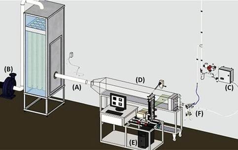
Figure 1 – Test Facility.

  <>2.2.       Operational and Geometrical Conditions

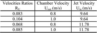
In the test facility, experiments were realized for two different initial velocities in the jet and in the chamber, which are presented in Table 1. This setup provides four different velocities ratios, which are presented in Table 2.

Table 1: Initial velocities in the jet and in the chamber.

 

Table 2: Velocities ratios.

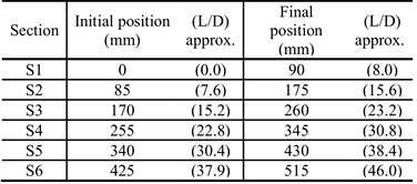
The experiments were developed at 25 °C. The PIV measurements were taken in the same horizontal plane, as showed in Figure 2. The measurement region is 510 mm length x 110 mm width, which is subdivided in six sections with 90 mm length x 110 mm width (Figure 2). The first (S1) and last (S2) coordinate sections are presented in Table 3, with the others sections. After calibration of the 2D-PIV system, 1000 frames were taken in the measuring region with a time step of 150 µs. Thus, two different axial positions were selected to investigate the radial profiles in terms of mean velocity and turbulence kinetic energy. These positions are located at L/D=25 and L/D=37.5. The geometrical conditions are presented in Figure 2, where D is the nozzle diameter.

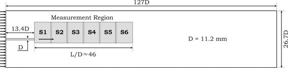
Figure 2 – Geometrical conditions and measurement region.

Table 3 – Sections for the experimental measurements.

  2.3.      Numerical Simulations

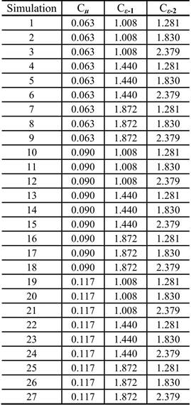
The objective of this study is to investigate the behavior of RSM-SSG model in a confined coaxial jet flow for different velocity ratios, changing the default values of some parameters of the model. In this way, the numerical simulations were performed varying the C_µ, C_ε-1 and C_ε-2 parameters in +30% and –30% of its default values.

In order to achieve this objective, an experimental design of three factors at three levels was performed, which is presented in Table 4.

Table 4 – Design of experiments.

The numerical simulations were conducted by a CFD commercial package, the FLUENT 13. The geometrical grid used in these simulations consists in approximately 291,640 hexahedral elements. The advection scheme used in the simulations was High Resolution due to the strong convective component of the gas transport. The convergence criterion for all cases was 10^–4 in the residual norm. The iterations were solved with a time step size of 10^–4 s, totalizing 5 seconds of real time simulation.

The boundary conditions for physical frontiers of the coaxial confined jet flow are:

·          Inlet (Chamber and Jet): It is adopted uniform and constant properties for the gas flow with an initial velocity condition.

·          Outlet: Constant pressure with continuity conditions for all flow properties.

·          Wall: No-slip conditions and wall logarithm function for the turbulent properties.

 

3.      RESULTS AND DISCUSSIONS

The numerical results of the axial mean velocities were compared with experimental data and analyzed by means of a criteria known as integrated absolute value of the error (IAE), where the set-point is the experimental data. The simulations results for the axial mean velocity are presented in Table 5.

Table 5 – Value of the errors determined by IAE criterion for the axial mean velocity.

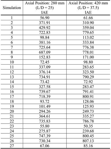
In the Table 5 it is possible to observe that the results to the simulations 1, 10, 23 and 27 are closer to the experimental data in relation to the default results (simulation 14) than the others simulations. These four results are selected to be analyzed in graphical form in terms of mean axial velocity profiles and turbulence kinetic energy profiles, as seen in Figure 3 and in Figure 4, respectively, for two different axial positions.

     

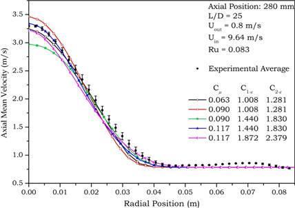
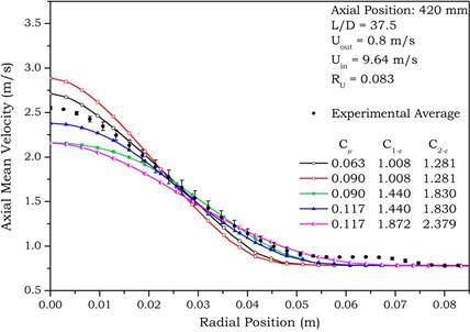
Figure 3 – Axial mean velocity profiles for two different axial positions.

In Figure 3 it is possible to observe that the best numerical result is obtained when the C_µ parameter is set to +30% to its default value and the two other parameters are fixed in default values (blue line). Extending this analysis, Figure 4 presents the turbulence kinetic energy profiles. For both axial positions it is possible to observe that the simulation with the default values parameters presented better result, however the simulation result which the C_µ parameter is adjusted in +30% to default value is also close to the experimental data, mainly at the L/D=37.5.

      

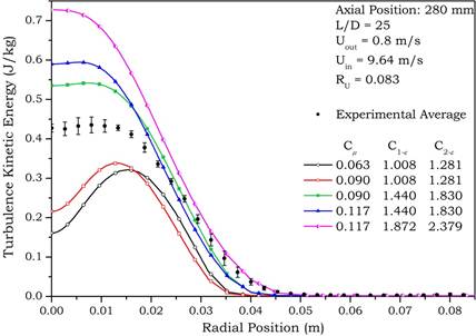
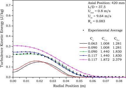
Figure 4 – Turbulence kinetic energy profiles for two different axial positions.

These 27 numerical simulations were also performed for the others velocities ratios and the results obtained were similar to those previously presented.

 

4.      CONCLUSIONS

The 27 simulation results are compared with PIV experimental data and the results showed that the best is obtained when the C_µ parameter is modified default value (0.09) to a value 30% above, i.e., for 0.117. These results indicate that the parametric sensibility analysis is a tool that can be used to determine the best fit for model parameters analysis.  

 

REFERENCES

Decker, R.K.; Buss, L.; Wiggers, V.R.; Noriler, D.; Reinehr, E.L.; Meier, H.F.; Martignoni, W.P.; Mori, M., (2011), Numerical Validation of a Coaxial and Confined Jet Flow, Chemical Engineering Transactions, 24, 1459-1464.  

Lin C.A., (1998), Modeling a confined swirling coaxial jet. Center for Turbulence Research, Annual Research Briefs.

Mahmoud H., Kriaa W., Mhiri H., Le Palec G. and Bournot P., (2010), A numerical study of a turbulent axisymmetric jet emerging in a co-flowing stream, Energy Conversion and Management, 51, 2117–2126.