
Data reconciliation comprises an important set of tools for data quality improvement. By removing always-present random measurement noise, one seeks to process the data so that the transformed data are an improved representation of the measured variables. Most often, this involves projection, filtering, or smoothing steps (e.g., Narasimhan & Jordache, 1999; Vachhani et al., 2005, 2006). Data reconciliation can be based on mechanistic models (white box, Venkatasubramanian et al., 2003a), empirical models (black box, Venkatasubramanian et al., 2003b, or a combination of both (gray box). This work is focused on data reconciliation methods that rely on mechanistic process understanding (white box data reconciliation).
A majority of the data reconciliation literature is concerned with the application of equality constraints as a way to improve the accuracy of the available measurements. In this case, data reconciliation is interpreted geometrically as a projection to a plane or manifold. The application of linear and nonlinear equality constraints for data reconciliation has been studied in great detail already (Tamhane & Mah, 1985; Crowe, 1996; Veverka & Madron, 1997; Romagnoli & Sanchez, 1999).
The application of inequality constraints has been studied as well. An early example is found in Narasimhan & Harikumar (1993) where knowledge about the feasible range of values for a measured process state is accounted for. Vachhani et al. (2006) proposed a method for dynamic data reconciliation based on the unscented Kalman filter, thereby enabling the application of inequality constraints into an online data reconciliation method. More recently, special attention has been given to the incorporation of prior knowledge about function and signal shapes to optimally describe or reconcile time series data (Villez et al., 2013; Villez & Habermacher, 2016; Derlon et al., 2017; Vertis et al., 2017; Masic et al, 2017; Srinivasan et al., 2017). Most typical is that the data analysis is enhanced by incorporation of prior knowledge about the signs of the first and second derivative of the fitted function or the data series.
The application of inequality constraints offers several advantages. For instance, in Narasimhan & Harikumar (1993) and Srinivasan et al. (2017) the improved accuracy of the reconciled data is the principal motivation to consider inequality constraints. In Villez & Habermacher (2016), shape constraints lead to the formulation of a lack-of-fit statistic. Vertis et al. (2016) mainly motivate the application of shape constraints as a way to differentiate time series data without risk of noise amplification (Bhatt et al., 2012) in turn enabling a reasonable guess of parameter values in kinetic models. A similar strategy to initialize parameter estimation is deployed in Masic et al. (2017).
The data reconciliation literature implicitly incorporates the idea that any prior knowledge should be applied during the data reconciliation process. This is based on the observation that application of knowledge-based equality and inequality constraints invariably improves the accuracy of the reconciled data as long as the applied constraints are correctly assumed for the data-generating process. The impact of using reconciled data, e.g. during model parameter estimation, has not been studied in detail yet. In this work it is demonstrated that data reconciliation with inequality constraints can induce significant bias during model parameter estimation.
2. Methods
The utility of data reconciliation is studied by means of a simple model parameter estimation problem. To this end, a batch experiment involving a single equilibrium reaction with two species, A and B, is repeatedly simulated. The simulated rate laws are linear in the consumed species concentrations for both directions of the reaction. Consequentially, the net reaction can be described by a kinetic rate law which exhibits two parameters: the reaction rate coefficient (k1=1 mol/L.h) and the equilibrium parameter (k2=0.2). The concentration of A is measured at regular intervals. The data collected in each experiment are first reconciled based on a monotonicity constraint and then used for parameter estimation. In parallel, the same data are also used for parameter estimation without any data reconciliation. In both cases, the initial process conditions and the kinetic rate law structure are assumed known. This complete procedure is repeated 10000 times to investigate the effects of data reconciliation in the parameter estimates.
3. Results
3.1 Simulation
Figure 1 displays the simulation results for a single batch experiment. One can see that the concentration of species A decreases with time from its initial value (1 mol/L) towards its equilibrium value (0.2 mol/L). Noisy measurements of the concentration of species A are obtained every 5 minutes during the 7-hour experiment.
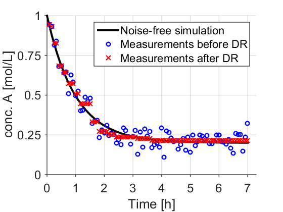
Figure 1: A single batch experiment – Black line: simulated concentration; Blue circles: Measurements before data reconciliation; Red crosses: Measurements after data reconciliation.
3.2 Data reconciliation
Reconciled measurements are obtained by computing concentrations that are close as possible to the original measurements in the least-squares (WLS) sense while satisfying isotonicity (non-strictly increasing). This monotonicity constraint is implemented as a positivity constraint for the point-wise differences between consecutive concentration measurements. Thus, the data reconciliation problem is a convex quadratic program with linear inequality constraints. Figure 1 displays the reconciled concentration measurements of species A. One observes that the reconciled measurements are generally closer to their true values and that –as expected- they increase with time.
Figure 2 shows the cumulative density of the obtained root mean squared error (RMSE) with error defined as the deviation between a measurement and its true noise-free value. As one can see, data reconciliation improves the obtained accuracy.
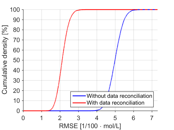
Figure 2: Accuracy of the measurements – Empirical cumulative density of the RMSE before and after data reconciliation.
3.3 Parameter estimation
Both kinetic rate law parameters are estimated simultaneously with both the unreconciled and reconciled measurements and for each simulated experiment separately. To this end, the parameter estimates are adjusted so that the simulated concentrations are as close as possible to the (unreconciled or reconciled) measurements in the least-squares sense. The results of this can be seen in Figure 3. Individual parameter estimates are shown for the first 250 experiments. The results of the complete Monte Carlo simulation are summarized by the mean parameter vector and the variance-covariance matrix computed from all parameter estimates. Figure 3 shows the 99% confidence ellipsoids according to an assumed multivariate normal distribution for the parameter estimates. Most importantly, one can see that the application of data reconciliation leads to a shift of the parameter estimates away from their ground truth values. In contrast, fitting the model to the unreconciled data directly does not induce such an effect and delivers parameters that are practically unbiased, i.e. their average is very close to the true parameter values.
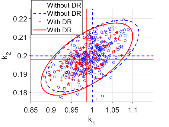
Figure 3: Accuracy of the parameter estimates – Blue circles: Parameter estimates with raw data; Blue dashed lines: mean and 99% confidence region for the parameter estimates with raw data; Red crosses: Parameter estimates obtained with reconciled data; Red full lines: mean and 99% confidence region for the parameter estimates obtained with reconciled data.
4. Conclusions
Data reconciliation with inequality constraints has been advocated as a generally applicable method to improve the accuracy of experimental data. In this study, it is shown with a simple simulation study that improved accuracy can come at a price when using the reconciled data for their ultimate purpose. Indeed, the parameter estimation study show that data reconciliation induces a biasing effect during parameter estimation. This is explained by the fact that (i) the reconciled data are distributed according to truncated multivariate normal distribution and (ii) the least-squares parameter estimation procedure assumes a multivariate normal distribution. So far, no data reconciliation method has been proposed that automatically accounts for this discrepancy. This, in part, explains why using the unreconciled data during parameter estimations leads to the best parameter estimates.
References
Bhatt N, Kerimoglu N, Amrhein M, Marquardt W, Bonvin D. Chemical Engineering Science. 2012;83:24-38.
Crowe C M. Journal of Process Control. 1996;6:89-98.
Derlon N, Thürlimann C M, Dürrenmatt D J, Villez K. Water Research. 2017;114:327-337.
Masic A, Srinivasan S, Billeter J, Bonvin D, Villez K. Computers & Chemical Engineering. 2017;99:96-105.
Narasimhan S, Harikumar P. Computers & Chemical Engineering. 1993;17:1115-1120.
Narasimhan S, Jordache C. Data reconciliation and gross error detection: An intelligent use of process data Gulf Professional Publishing. 1999.
Noorman H J, Romein B, Luyben K Ch A M, Heijnen J J. Biotechnology and Bioengineering. 1996;49:364-376.
Romagnoli J A, Sanchez M C. Data processing and reconciliation for chemical process operations (Vol. 2). Academic Press 1999.
Srinivasan S, Billeter J, Narasimhan S, Bonvin D. Computers & Chemical Engineering. 2017;101:44-58.
Tamhane A C, Mah R S. Technometrics. 1985;27:409-422.
Vachhani P, Rengaswamy R, Gangwal V, Narasimhan S. AIChE Journal. 2005;51:946-959.
Vachhani P, Narasimhan S, Rengaswamy R. Journal of Process Control. 2006;16:1075-1086.
Venkatasubramanian V, Rengaswamy R, Yin K, Kavuri S N. Computers & Chemical Engineering. 2003a;27:293-311.
Venkatasubramanian V, Rengaswamy R, Kavuri S N, Yin K. Computers & Chemical Engineering. 2003b;27:327-346.
Vertis C S, Oliveira N M C, Bernardo F P. Computer Aided Chemical Engineering. 2016;38:2121-2126.
Veverka V V, Madron F. Material and energy balancing in the process industries: From microscopic balances to large plants (Vol. 7). Elsevier 1997.
Villez K, Venkatasubramanian V, Rengaswamy R. Computers & Chemical Engineering. 2013;58:116-134.
See more of this Group/Topical: Computing and Systems Technology Division